Core: Physical Object
Description
The Physical Object is the base class of all objects that exist within the simulation that have some form of physical modelling applied. A physical object is a custom Component that can have a mass, have dynamical properties and can be attached to spacecraft or ground stations. Physical objects in their raw form do not have any functionality, but provide useful data for fetching and updating the mass properties and transforms relative to their parent. With the exception of flight software, almost all components that are attached to a spacecraft are physical objects. The spacecraft itself also derives from a physical object.
Module Implementation
A user can adjust two transformation properties on the physical object:
- \({}^P\textbf{r}_{LP}\): The position of the object relative to its parent in the parent’s rotational frame \(P\)
- \(\mathrm{DCM}_{LP}\): The rotation of the object relative to its parent in the parent’s rotational frame \(P\)
These values internally update the transformation matrix \(T_{PL}\), which handles the rotational and position frame change between the parent \(P\) and component \(L\) frames. Note that \(T_{PL}.\mathrm{DCM} = \mathrm{DCM}_{LP}\), as the DCM (direct-cosine-matrix) representing the same rotation is the transpose of the rotation part of \(T_{PL}\). In the case of the highest parent, \(B\), then the local position and rotation are relative to the inertial frame \(N\), which would be in the centre of the zero-base set up on the Universe system (defaulted to the Earth). The following diagram illustrates how the various objects can be parented and how their frame changes:
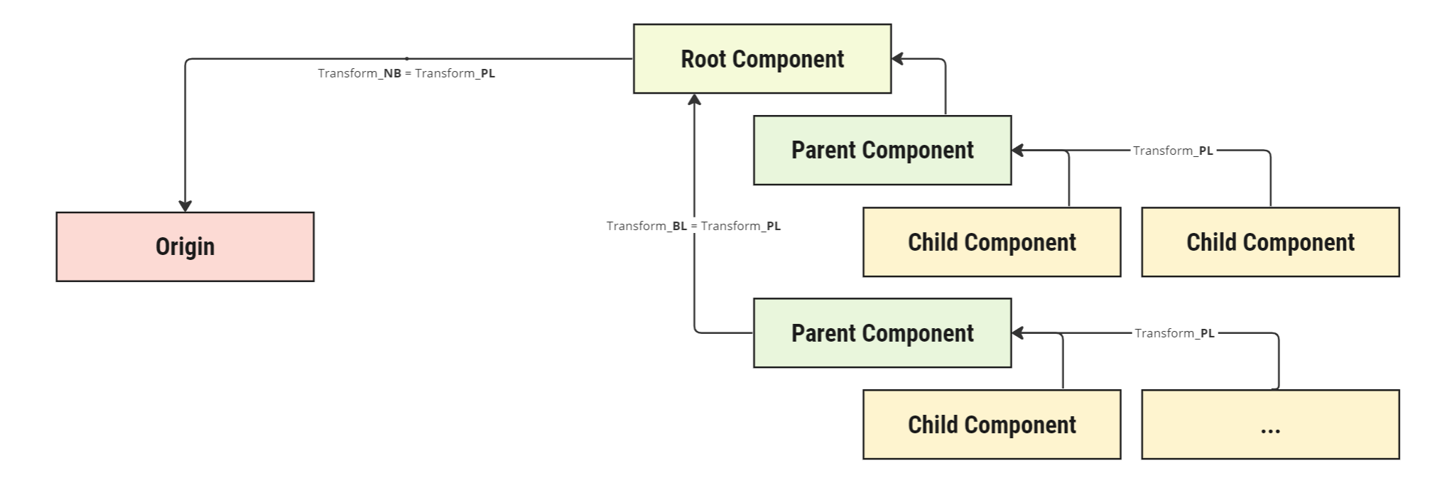
In this case, the root component is the topmost parent of the structure (usually the spacecraft or ground station). Each component that is attached to another component can have components attached to it and any number of components can be attached to each component. There is no restriction or limitation to the number of components or chains that can occur on a component hierarchy.
The object can retrieve these values in different reference frames, without being modified. For example, regardless of which location the component is placed in. There are four reference transformations that are available:
| Transform | From Frame | To Frame | Editable |
|---|---|---|---|
| Transform_PL | Parent \(P\) | Component \(L\) | Yes |
| Transform_BL | Body \(B\) | Component \(L\) | No |
| Transform_NL | Inertial \(N\) | Component \(L\) | No |
| Transform_NB | Inertial \(N\) | Body \(B\) | No |
Although the three other transforms are available to be read from on the components, only the local transform is editable. Each component local transform can have its rotational matrix (DCM) and position edited. To calculate the body-component transform, \(\mathrm{T}_{BL}\), then a recursive lookup is applied to determine the transformation from the component frame \(L\) to the root body frame \(B\):
where the chain will continue to look up the component stack until the parent = null, in which the final \(\mathrm{T}_{PL}\) value is used. The root \(\mathrm{T}_{PL}\) is the transformation from the inertial frame. In the root’s case only, then:
Similarly, for the first level parent (a component attached directly to the root object or spacecraft), the body transform is equivalent to the parent transform:
This is not the case for a second-level component, which is attached to a component that is not the root component of the hierarchy. To determine the inertial transformation of any component relative to the inertial origin \(N\), then the chain transformations are used:
Along with the transformation properties, the physical object can also have mass properties attached to the component. By default, all values have an initial parameter and can be changed during the simulation:
| Property | Symbol | Definition | Value Type | Default Value |
|---|---|---|---|---|
| Mass | \(m\) | The mass of the component. | Double | 0 |
| Mass Dot | \(\dot{m}\) | The change in mass of the component over time. | Double | 0 |
| Center of Mass | \({}^L\textbf{r}_{LmL}\) | The centre of mass of the component in the component’s frame. | Vector3 | \([0, 0, 0]\) |
| Center of Mass Dot | \({}^L\dot{\textbf{r}}_{LmL}\) | The centre of mass changes over time in the component’s frame. | Vector3 | \([0, 0, 0]\) |
| Centre of Mass Prime | \({}^B{\textbf{r}'}_{LmB}\) | The centre of mass changes in the body frame of the component over time. | Vector3 | \([0, 0, 0]\) |
| Moment of Inertia | \({}^LI_{PntLm}\) | The moment of inertia in the component’s frame. | Matrix3 | \(I_{33}\) |
| Moment of Inertia Prime | \({}^LI'_{PntLm}\) | The rate of change of the moment of inertia is calculated relative to the body frame. | Vector3 | \(0_{33}\) |
These seven properties are used by a number of dynamical systems on the spacecraft, but not all are required to be edited for each component. However, each of these values is in terms of the component’s frame (\(Lm\)). The physical object does expose the calculations for the same parameters in the body frame \(B\) which can be calculated and returned, but not edited.
The moment of inertia values can also be transformed to the body frame \(B\) using the following equations:
where the \(\tilde{\textbf{r}}_{LmB}\) is the skew matrix from the local centre of mass of the component in the body frame and \(\tilde{\textbf{r}}'_{LmB}\) is the skew matrix from the local centre of mass prime of the component in the body fame. The transformation of the inertial matrix uses the parallel axis theorem to calculate the inertial tensor in the body frame.
For optimization and performance, a cache of the body frame transforms and mass properties are stored and only updated in a component in the hierarchy chain is changed or the component’s transform or mass properties are updated. The cache stores the data and if adjusted, a new cache of calculations will be stored and referenced. The cache uses the same functionality as above.