Software: LVLH Pointing

Description

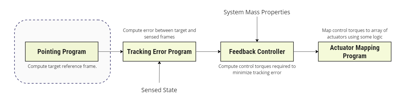
This module is designed to work as the pointing program in an ADCS software chain as shown in the figure below.

This module constructs an output reference frame \(\mathcal{R}\) that aligns with the Local-Vertical-Local-Horizontal (LVLH) reference frame \(\mathcal{L}: [\hat{i}_r, \hat{i}_h, \hat{i}_\theta ]\) where:

\(\hat{i}_r\): points radially outward in the direction that connects the centre of the planet with the parent object.

\(\hat{i}_h\): is defined normal to the orbital plane in the direction of the angular momentum

\(\hat{i}_\theta\): completes the right-handed triad.

Example Use Cases

• Compute the LVLH reference frame for pointing applications: Construct a reference frame commonly applied for nadir pointing operations e.g. Earth Observation.
• Supports navigation translation errors modelling: Accepts general navigation messages, which may provide body state estimations from sensors, flight computers, etc. or the actual body state directly from the parent spacecraft.

Module Implementation

Reference Frame Definition

This module assumes a standard reference frame, where \(\mathbf{R}_s\) is the position vector of the spacecraft in the inertial frame \(\mathcal{N}: [\hat{n}_1, \hat{n}_2, \hat{n}_3 ]\) and \(\mathbf{R}_p\) is the position vector of the celestial body in the inertial frame. The relative position and velocity of the spacecraft in the planet-centred inertial frame are then:

\[ \mathbf{r} = \mathbf{R}_s-\mathbf{R}_p \\ \mathbf{v} = \mathbf{v}_s - \mathbf{v}_p \]

The Hill frame orientation is then defined as:

\[ \hat{\mathbf{i}}_r = \frac{\mathbf{r}}{r}\\ \hat{\mathbf{i}}_h = \frac{\mathbf{r}\times \mathbf{v}}{rv}\\ \hat{\mathbf{i}}_\theta=\hat{\mathbf{i}}_h \times \hat{\mathbf{i}}_r \]

The direction cosine matrix that maps \(\mathcal{R}\) to \(\mathcal{N}\) is then \([RN] = [\hat{i}_r, \hat{i}_\theta, \hat{i}_h]\).

Reference Frame Angular Velocity Vector

The angular velocity of the original reference frame \(\mathcal{R}_0\) is \(\omega_{R_0/N}\). The angular rate and acceleration vectors are then defined by the true anomaly \(f\) of the orbit as:

\[ \omega_{R_0/N} = \dot{f} \hat{\mathbf{i}}_h = \frac{h}{r^2} \hat{\mathbf{i}}_h \\ \dot{\omega}_{R_0/N} = \ddot{f} \hat{\mathbf{i}}_h = -2 \frac{\mathbf{v} \cdot \hat{\mathbf{i}}_r}{r} \dot{f} \hat{\mathbf{i}}_h \]

The angular rate and acceleration in the output reference frame are then computed as:

\[ \omega_{R/N} = \omega_{R/R_0} + \omega_{R_0/N} = \dot{f} \hat{\mathbf{i}}_h \\ \dot{\omega}_{R/N} = \ddot{f} \hat{\mathbf{i}}_h \]

Expressed in the inertial frame:

\[ ^\mathcal{N}\omega_{R/N}=[NR] ^\mathcal{R}\omega_{R/N} \]

\[ ^\mathcal{N}\dot{\omega}_{R/N}=[NR] ^\mathcal{R}\dot{\omega}_{R/N} \]

where \([NR] = [RN]^T\).

References

[1] Hanspeter Schaub and John L. Junkins. Analytical Mechanics of Space Systems. AIAA Education Series, Reston, VA, 3rd edition, 2014.