Editor: Changing Integrators
Description
The simulation runs all components on a single time loop, where the time step is controlled by the user. Each component is ticked in the simulation in the order that the components were added. However, for dynamic objects, an integrator is used to step through the values within each state. Dynamic objects include any dynamic or state effector that has a property with a derivative. These include:
- Spacecraft
- Reaction Wheels
- Thrusters
- Fuel Sources
- Hinged Rigid Bodies
- Magnetic Torque Bars
- Any other component that inherits from
StateEffectororDynamicEffector
Although not every parameter within these components is integrated in this way, the step between each simulation timestep will take the state parameters and parse them through an integrator object. For example, the spacecraft’s position is stored as a state, with a derivative that is calculated (the velocity). The velocity is also stored as a state with the derivative calculated (the acceleration). Each step the integrator is called which subsequently invokes an integrator function that may update the state and derivative of any integrable properties multiple times per simulation tick. In the case of the RK4 integrator, these properties are updated 4 times per simulation call, meaning each derivative and state for every dynamic effector are calculated 4 times every simulation call.
As such, picking the correct integrator is a balance between simulation speed and the accuracy of numerical calculations. Typical single-spacecraft simulations can have a time improvement of up to 50% when switching the integrator from RK4 to Euler for example, with the downside of being numerically inaccurate with larger time-steps.
Switching Integrators
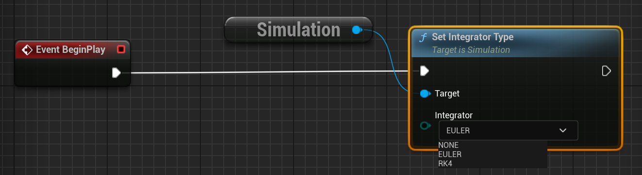
Nominal Editor allows the default integrator for a particular simulation to be changed between the options. This can be configured on the simulation system and must be done at each simulation level on the level blueprint. The integrator can be changed by calling Set Integrator Type on the Simulation System. This applies the integrator for all objects created after it is called. It cannot change the integrator for spacecraft that are already created.
Note
Setting the integrator type as NONE will use the default integrator for the simulation.
Runge-Kutter 4 (RK4)
The Runge-Kutta (RK4) method is a numerical technique used for solving ordinary differential equations. It is a fourth-order method, meaning that its local truncation error is on the order of \(h^5\), where \(h\) is the step size. RK4 is widely used because it strikes a good balance between accuracy and computational efficiency.
The general form of a first-order equation is:
where \(y\) is the unknown function of \(t\), and \(f(t, y)\) is a given function. The RK4 method iteratively estimates the solution \(y(t)\) at discrete time points \(t_0, t_1, t_2, ...\) by updating the solution using the following formula:
where:
- \(y_n\) is the approximation of \(y(t)\) at time \(t_n\)
- \(h\) is the step size
- \(k_1\) is the first estimate of the derivative at \(t_n\)
- \(k_2\) is the second estimate of the derivative at \(t_n + {h \over 2}\)
- \(k_3\) is the third estimate of the derivative at \(t_n + {h \over 2}\)
- \(k_4\) is the fourth estimate of the derivative at \(t_n\)
The formulas for \(k_1\), \(k_2\), \(k_3\) and \(k_4\) are defined as follows:
This method essentially takes four weighted estimates of the slope at different points and combines them to update the solution at each step. The accuracy of RK4 makes it a popular choice for solving differential equations such as the velocity and attitude of spacecraft.
Note
The RK4 integrator is the default integrator if left unchanged. This is the integrator for all other spacecraft if not changed or the default settings are not adjusted.
Euler
The Euler method is a simple numerical technique for solving ordinary differential equations. It is a first-order method, meaning that its local truncation error is on the order of \(h^2\), where \(h\) is the step size. The basic idea of the Euler method is to approximate the solution at each time step by using the derivative at the current time. The update formula is given by:
where:
- \(y_n\) is the approximation of \(y(t)\) at time \(t_n\)
- \(h\) is the step size
- \(f(t_n, y_n)\) is the derivative of \(y\) at time \(t_n\)
The formula is derived from the definition of the derivative:
By approximating the derivative with the finite difference \({\Delta y \over \Delta t}\), where \(\Delta y\) is the change in \(y\) and \(\Delta t\) is the change in \(t\) (in this case \(\Delta t = h\)), you get the Euler formula. While the Euler method is easy to implement, it has limitations, especially where accuracy is crucial. It tends to accumulate errors over time, and its accuracy is lower compared to higher-order methods like the RK4 method. Despite its limitations, the Euler method is still useful for solving simple ODEs when computational efficiency is not a primary concern.